Statistics and Probability for AI

1 Types of Data

Numerical Data: is data in the form of numbers

• Represents some sort of quantitative measurement (Heights of people, Page load times, Stock prices, etc.)
• Discrete Data (Integer based; often counts of some event)
• Continuous Data (Has an infinite number of possible values)

Categorical Data: is data that can be grouped into categories instead of being measured numerically

• Qualitative data that has no inherent mathematical meaning (Gender, Yes/No, Product Category)
• Number Category but dont have mathematical meaning

Ordinal Data: is mixture of numerical and categorical data

• Categorical data (Ratings on 1-5)

2 Mean, Median, and Mode

Mean: is the average of a data set is found by adding all numbers in the data set and then dividing by the number of values in the set.

import numpy as np

# normal distribution
# (mean, standard deviation, size)
incomes = np.random.normal(27100, 15000, 10000)

np.mean(incomes)

Result:

26996.83588058297

Median: is the middle number in a sorted list of numbers (either ascending or descending).

np.median(incomes)

Result:

27049.84671143801

Median: is the value that is the most repeatedly occurring in a given set.

import numpy as np
from scipy import stats

# Integer Random Generator
# (low, high, size)
ages = np.random.randint(18, 90, size=500)

stats.mode(ages)

Result:

ModeResult(mode=28, count=12)

3 Standard Deviation and Variance

Standard Devication (σ): is a measure of the amount of variation of a random variable expected about its mean.

Variance (σ²): is the expected value of the squared deviation from the mean of a random variable.

• Population Variance: σ² = ∑(Χ-μ)²/N
• Sample Variance: σ² = ∑(Χ-M)²/(n-1)

import numpy as np
import matplotlib.pyplot as plt

incomes = np.random.normal(100, 20, 10000)

plt.hist(incomes, 50)
plt.show()

Result:

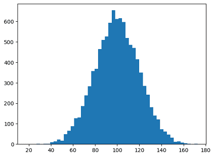
incomes.std()

Result: 20.075094748090326

incomes.var()

Result: 403.00942914480373

4 Probability Density Function

The Probability Density Function defines the probability function representing the density of a continuous random variable lying between a specific range of values.

(For the discrete data, it will be Probability Mass Function.)

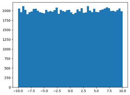
• Uniform Distribution: is a flat constant probability of a value occuring within a given range.

import numpy as np
import matplotlib.pyplot as plt

# unform(start, end, value)
values = np.random.uniform(-10.0, 10.0, 100000)

plt.hist(values, 50)
plt.show()

Result:

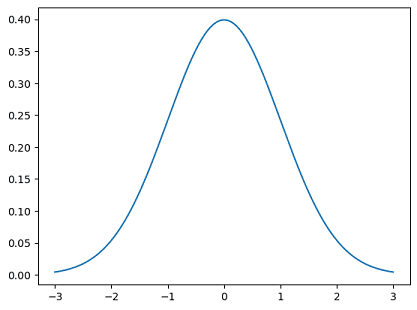
• Normal/Gaussian Distribution:

from scipy.stats import norm
import matplotlib.pyplot as plt

x = np.arange(-3, 3, 0.001)
plt.plot(x, norm.pdf(x))

Result:

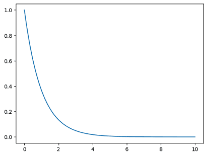
• Exponential Distribution:

from scipy.stats import expon
import matplotlib.pyplot as plt

x = np.arange(0, 10, 0.001)
plt.plot(x, expon.pdf(x))

Result:

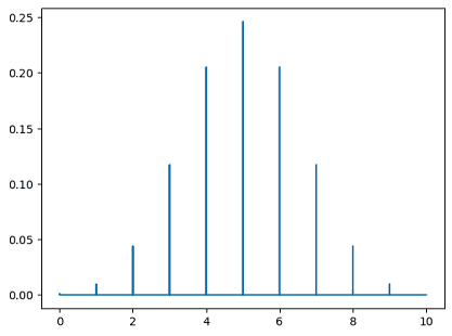
• Binomial Probability Mass Function:

from scipy.stats import binom
import matplotlib.pyplot as plt

n, p = 10, 0.5
x = np.arange(0, 10, 0.001)
plt.plot(x, binom.pmf(x, n, p))

Result:

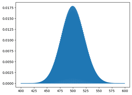
• Poisson Probability Mass Function:

from scipy.stats import poisson
import matplotlib.pyplot as plt

mu = 500
x = np.arange(400, 600, 0.5)
plt.plot(x, poisson.pmf(x, mu))

Result:

5. Percentiles and Moments